Factorization Machines for Recommendation Systems

As a Data Scientist that works on Feed Personalization, I find it it important to stay up to date with the current state of Machine Learning and its applications. Most of the time, using some of the better-known recommendation algorithms yields good initial results; however, sometimes a change in the model is essential to provide customers with that extra boost that helps increase engagement in their apps. This is how we ended up reading and researching the use of Factorization Machines (FM) to improve our personalization engine.

This blogpost will provide brief explanation of Factorization Machines (FM) and their applications to the cold-start recommendation problem. FM models are at the cutting edge of Machine Learning techniques for personalization; they have proven to be an extremely powerful tool with enough expressive capacity to generalize methods such as Matrix/Tensor Factorization and Polynomial Kernel regression.

The Model

Most recommendation problems assume that we have a consumption/rating dataset formed by a collection of _(user, item, rating_) tuples. This is the starting point for most variations of Collaborative Filtering algorithms and they have proven to yield nice results; however, in many applications, we have plenty of item metadata (tags, categories, genres) that can be used to make better predictions. This is one of the benefits of using Factorization Machines with feature-rich datasets, for which there is a natural way in which extra features can be included in the model and higher order interactions can be modelled using the dimensionality parameter d. For sparse datasets, a second order FM model suffices, since there is not enough information to estimate more complex interactions. Here is what a second order FM model looks like: 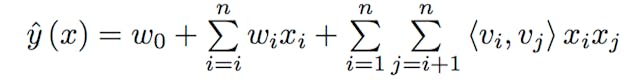Where the v's represent k-dimensional latent vectors associated with each variable (i.e. users and items) and the bracket operator represents the inner product. For anyone that has studied Matrix Factorization models, the previous equation should look familiar: it contains a global bias as well as user/item specific biases and includes user-item interactions. Following Steffen Rendle's original paper on FM models, if we assume that each x(j) vector is only non-zero at positions u and i, we get classic Matrix Factorization model: The main difference between the previous two equations is that FM introduces higher order interactions in terms of latent vectors that are also affected by categorical or tag data. This means that the models go beyond co-occurrences in order to find stronger relationships between the latent representations of each feature. Following the original implementation of Factorization Machines, the training data should be structured as follows: 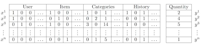We will use tffm, an implementation of Factorization Machines in TensorFlow, and pandas for pre-processing and structuring the data. FM models work with categorical data represented as binary integers, if you are already using Pandas Data Frames I recommend that you use the get_dummies method to transform all columns with categorical data. I will use the RecSys 2015 challenge dataset to illustrate how to fit a FM model. The data contains click and purchase events for an e-commerce site, with additional item category data, you can download it here (275MB). We will be using youchoose-buys.dat and youchoose-clicks.dat.

Example

To get started, you’ll need the following Python packages:

pip install pandas==0.19.2
pip install tensorflow==0.12.1
pip install numpy==1.12.0
pip install scikit-learn==0.18.1
pip install tqdm==4.11.2
pip install scipy==0.17.0

You will also install tffm and run your code inside the main folder

git clone https://github.com/geffy/tffm.git
cd tffm

Here's a link to the full code of our example, in case you want to skip the explanations. In order to make full use of the categories and expanded historical data , we need to load and convert the data into the right format.

Ready to integrate? Our team is standing by to help you. Contact us today and launch tomorrow!

import pandas as pd
from collections import Counter
import tensorflow as tf
from tffm import TFFMRegressor
from sklearn.metrics import mean_squared_error
from sklearn.model_selection import train_test_split
import numpy as np
# Loading datasets'
buys = open('yoochoose-buys.dat', 'r')
clicks = open('yoochoose-clicks.dat', 'r')
initial_buys_df = pd.read_csv(buys, names=['Session ID', 'Timestamp', 'Item ID', 'Category', 'Quantity'],
                              dtype={'Session ID': 'float32', 'Timestamp': 'str', 'Item ID': 'float32',
                                     'Category': 'str'})
initial_buys_df.set_index('Session ID', inplace=True)
initial_clicks_df = pd.read_csv(clicks, names=['Session ID', 'Timestamp', 'Item ID', 'Category'],
                                dtype={'Category': 'str'})
initial_clicks_df.set_index('Session ID', inplace=True)
# We won't use timestamps in this example
initial_buys_df = initial_buys_df.drop('Timestamp', 1)
initial_clicks_df = initial_clicks_df.drop('Timestamp', 1)
# For illustrative purposes, we will only use a subset of the data: top 10000 buying users,
x = Counter(initial_buys_df.index).most_common(10000)
top_k = dict(x).keys()
initial_buys_df = initial_buys_df[initial_buys_df.index.isin(top_k)]
initial_clicks_df = initial_clicks_df[initial_clicks_df.index.isin(top_k)]
# Create a copy of the index, since we will also apply one-hot encoding on the index
initial_buys_df['_Session ID'] = initial_buys_df.index

As we mentioned earlier, we can introduce historical engagement data into our FM model. We will use some group_by magic to generate a history profile of all user's engagement.

# One-hot encode all columns for clicks and buys
transformed_buys = pd.get_dummies(initial_buys_df)
transformed_clicks = pd.get_dummies(initial_clicks_df)
# Aggregate historical data for Items and Categories
filtered_buys = transformed_buys.filter(regex="Item.*|Category.*")
filtered_clicks = transformed_clicks.filter(regex="Item.*|Category.*")
historical_buy_data = filtered_buys.groupby(filtered_buys.index).sum()
historical_buy_data = historical_buy_data.rename(columns=lambda column_name: 'buy history:' + column_name)
historical_click_data = filtered_clicks.groupby(filtered_clicks.index).sum()
historical_click_data = historical_click_data.rename(columns=lambda column_name: 'click history:' + column_name)

Once we have the historical data we expand and embed it in the original set.

# Merge historical data of every user_id
merged1 = pd.merge(transformed_buys, historical_buy_data, left_index=True, right_index=True)
merged2 = pd.merge(merged1, historical_click_data, left_index=True, right_index=True)

And feed it into the FM model, we will generate to test sets, one with full information about the user's purchase and click history and the other one only with category metadata.

# Create the MF model, you can play around with the parameters
model = TFFMRegressor(
    order=2,
    rank=7,
    optimizer=tf.train.AdamOptimizer(learning_rate=0.1),
    n_epochs=100,
    batch_size=-1,
    init_std=0.001,
    input_type='dense'
)
merged2.drop(['Item ID', '_Session ID', 'click history:Item ID', 'buy history:Item ID'], 1, inplace=True)
X = np.array(merged2)
X = np.nan_to_num(X)
y = np.array(merged2['Quantity'].as_matrix())
# Split data into train, test
X_tr, X_te, y_tr, y_te = train_test_split(X, y, test_size=0.2)
#Split testing data in half: Full information vs Cold-start
X_te, X_te_cs, y_te, y_te_cs = train_test_split(X_te, y_te, test_size=0.5)
cold_start = pd.DataFrame(X_te_cs, columns=merged2.columns)
# What happens if we only have access to categories and no historical click/purchase data?
# Let's delete historical click and purchasing data for the cold_start test set
for column in cold_start.columns:
    if ('buy' in column or 'click' in column) and ('Category' not in column):
        cold_start[column] = 0
# Compute the mean squared error for both test sets
model.fit(X_tr, y_tr, show_progress=True)
predictions = model.predict(X_te)
cold_start_predictions = model.predict(X_te_cold)
print('MSE: {}'.format(mean_squared_error(y_te, predictions)))
print('Cold-start MSE: {}'.format(mean_squared_error(y_te_cold, predictions)))
model.destroy()
# Fun fact: Dropping the category columns in the training dataset makes the MSE even smaller
# but doing so means that we cannot tackle the cold-start recommendation problem

Here are the MSE results:

Full Information MSE: 0.00644224764093

Cold-start MSE: 3.09448346431

The experimental results are pretty good considering that we have used a relative small dataset to fit our model. As expected, it is easier to generate predictions if we have access to the full information setting with item purchases and clicks, but we still get a decent predictor for cold-start recommendations using only aggregated category data.

Feel free to contact us of you are interested in learning more about how Personalization can help improve retention and conversion in your app.