

RocksDB is a high-performance, embeddable storage engine originally developed by Facebook and is now widely adopted across the tech industry and used at Stream as a data storage engine. This powerful database solution has gained significant traction due to its exceptional speed, reliability, and versatility and is used by large companies such as LinkedIn, Meta, Google and Yahoo. In this article, we'll delve into the innovative design principles behind RocksDB, exploring how its architecture enables it to excel in a variety of demanding environments.
A Brief Overview of RocksDB
RocksDB saw the day in …. as a fork of LevelDB, a storage engine developed by Google and embedded in Google’s Big Table. It’s optimised for flash and SSD storage hardware and is based on “Log Structured Merge Trees” - LSM Trees for short. Don’t worry for now, we will present LSM trees in more detail afterwards. RocksDB has 3 main selling points: Embeddable, Customizable and Performant.
Embeddable Storage Engine
RocksDB is NOT a full database storage like MySQL or PostgreSQL, it doesn’t have any capability to parse SQL queries and doesn’t aim to do so. It’s a storage engine that can be used by other databases and other products easily. The main idea behind this concept of embeddability is the integration of RocksDB directly into the application server, eliminating the need for a separate database server. This approach offers several key advantages:
- Reduced latency: By eliminating network communication between the application and database, data access becomes significantly faster and latency will be dominated by IO speeds instead of network speed.
- Simplified architecture: Microservices based architectures are great but applications don’t always need the complexity that comes with it. Sometimes a monolith is better than a decoupled design as reported by AWS, and RocksDB promotes a simple monolith architecture.
- Better data locality: For applications that run on resource constrained edge devices, having data locally is more efficient than storing it in a separate server, particularly with limited data bandwidth.
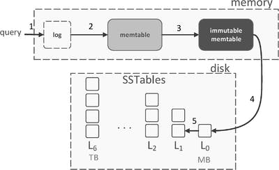
Meta has a great talk on Youtube on how RocksDB was designed and explains the decision behind making the project embeddable. Below is a diagram taken from the talk.

Customised to the Bone
RocksDB is a highly customizable storage engine, it’s designed in a way that all components are pluggable and can be exchanged with other components that are custom-developed by other entities. For instance, you can define your own format for the Memtable and SSTable, you can also configure how and when the data is flushed from memory to the disk, how the compaction works, fine tune the read/write amplification and even plug in your own compression algorithm. Don’t worry if you don’t understand terms like SSTable, compaction, etc. We will explain what these concepts are in the LSM section.
This flexibility allows RocksDB to be used in a wide range of use-cases from simple data storage to real-time streaming. In fact, both Kafka Streams and Apache Flink, two notorious technologies for data streaming, use RocksDB as a storage backend. Similarly, several databases use RocksDB as a storage engine, such as CockroachDB (although they moved to a Go based fork recently, known as PebbleDB), MyRocks (MySQL with RocksDB, used at Meta) and TiKV.
High Performance
RocksDB is based on LSM trees and is very fast, especially when used with the right hardware such as flash drives and SSD. The architecture of LSM trees-based databases like RocksDB is optimised for massive read-write operations on these storage hardware. We will better understand why it’s the case when we present LSM trees in more detail in this article. Unlike its predecessor, LevelDB, RocksDB implements a set of features that makes it really performant.
For instance, RocksDB implements Bloom filters, a probabilistic data structure that are used to quickly determine if a key might exist in a file (SSTable in this case), before performing a search on that file, this makes scans more efficient by reducing unnecessary I/O operations for keys that don’t even exist in a file. Another example is the use of concurrency by RocksDB. The storage engine takes advantage of multicore CPUs to perform read and write operations simultaneously without stalling much, this gives it a good advantage over previous LSM Tree-based databases like LevelDB that were single-threaded.
RocksDB Architecture
We will now delve deeper into how RocksDB works internally and explain some concepts of LSM Trees, the underlying data structure behind RocksDB. We will then present some things that RocksDB does differently and how it improves on LevelsDB.
LevelDB at Its Core
An important part of RocksDB architecture comes from LevelDB by Google. LevelDB was released in 2011 and had the same design principles as Google’s BigTable data store, it’s based on Log Structured Merge TRees (LSM Trees) as the underlying data-structure as presented in the figure below (see next section for more details on LSM Trees). Although LevelDB was a cornerstone technology in the development of other fast LSM based like RocksDB it lacked parallelism and suffered from a high write amplification due to how LSM trees store data on disk, we will delve into more details about how RocksDB improves upon these issues in the rest of this article.
A Short Introduction to LSM Trees
Traditional relational databases use a data structure known as B-trees (and B+ trees) to store and index data at a low level, these data structures are great for reads but can result in more overhead/cost for writes due how the tree is balanced and the insert/update algorithm on these trees. For an application that performs a lot of write operations its best to adopt a structure that is optimised for writes: Log structured merge trees or LSM trees for short is a suitable data structure that can offer low write latencies with a high throughput (number of write ops per second).
A Log-Structured Merge Tree is a data structure optimised for write-heavy workload. It organises data by initially writing updates to an in-memory structure (often known as Memtable), which is later flushed to disk in a sequential, append-only manner, creating sorted files called SSTables, these SSTables are immutable and structured similarly to a write ahead log (WAL) in traditional databases, hence the “Log Structured” term in LSM. This minimises disk I/O and improves write performance.
It is important to note that these SSTables are immutable, so deleting data or updating data will not really change the data in place, instead it will be marked as a new entry. Over time, older SSTables are merged and compacted regularly, during this process, stalled data is removed. This helps in maintaining efficiency and reducing storage space. Below is an example of an LSM tree from this great bytebytego video on the topic.
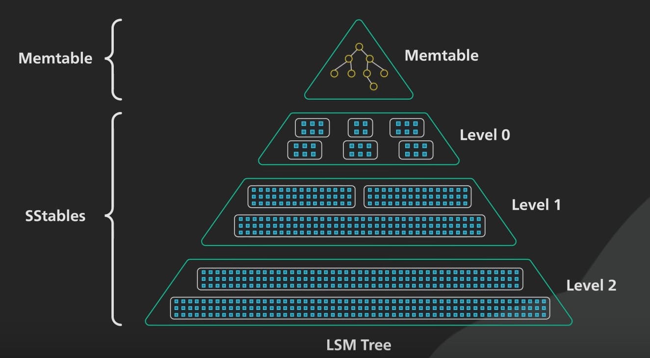
The three core components of LSM Trees:
- Memtables: These are in-memory data structures that are very fast to write to and read from, you can think of it as similar to a cache. Every query to RocksDB interact with the Memtable first, the new data is kept in memory until it reaches a certain configurable threshold (4MB in LevelDB) and then it’s flushed into the disk in a special format known as an SSTable.
- SSTable: SSTables is a concept found in Google BigTable and HBase, they are immutable files on the disk that are sorted in a similar fashion to a write-ahead logs. Over time, frequent writes to the Memtable will result in accumulating several SSTables, some of these files will hold outdated/stale data. Thankfully, LSM trees have a process known as compaction which we will discuss next.
- Compaction: The M in LSM refers to “Merge”: the SSTables are regularly merged together in a process named “compaction”. Compaction combines and sorts the SSTables, discarding deleted entries and consolidating data. There are several compaction algorithms, which can be classified into two families: Levelled Compaction introduced by LevelDB and Tiered Compaction which is used by RocksDB by default.
Compaction in RocksDB
Since LSM trees are the core data structure of RocksDB, the storing engine performs compaction regularly with some differences. First, instead of performing a simple tiered compaction where data in the MemTable is flushed to the disk directly into an SSTable, the compaction in RocksDB is level-based where the data on the disk is organized in ordered levels: Level 0, Level 1, Level 2. When data is flushed from the disk it is stored in Level 0 until it reaches a certain threshold, then it’s merged into Level 1 with a higher size threshold as represented in this figure from RocksDB wiki:

An important improvement of RocksDB is the ability to perform compaction in parallel, speeding up the process on instances with multi-core CPUs; the number of simultaneous compaction jobs can be also tuned in RocksDB configuration.
Unlike standard LSM trees where compaction starts when SSTables reach a certain size, RocksDB allows for a more flexible approach to trigger compaction. It can use the standard size limit as a trigger or monitor other metrics. For example, if we notice that write amplification becomes too high, it might be time to trigger a compaction to reduce data on the disk. RocksDB lets users configure these settings to better control when compaction occurs. RocksDB wiki has an insightful entry on compaction which I recommend reading if you want to understand how the merging process works within the storage engine.
Read & Write Amplification in RocksDB
Before delving into how RocksDB substantially improves read and write amplification (and space amplification, let’s first define what these are:
- Read Amplification: Read amplification refers to the amount of data that needs to be read from storage to satisfy a single read request. In simple terms, it's the ratio of the amount of data read from the storage device to the amount of data actually requested by the user. For example, if you need to read 1 KB of data, but the database system has to read 10 KB from disk to find and retrieve that 1 KB, the read amplification is 10x.
- Write Amplification: Similar to read amplification, write amplification refers to the amount of data that needs to be written to disk when performing a single write in the database. For instance, if we write 1 KB of data to the database and this result in 8 KB being written to disk due to moving data around and rewrites the resulting write amplification is 8x.
- Space Amplification: Space amplification refers to the amount of additional storage overhead required beyond the raw size of the data. This overhead can come from indexes, meta-data and stale data.
It’s usually only possible to optimise two of the three above, in this article we will focus on read and write amplification and how it’s optimised (reduced) by RocksDB.
Why does it matter?
Modern SSDs lifetime is limited by a certain number of write cycles, so having a high write amplification means more write cycles which directly degrade the SSD lifetime. This is an important issue in storage systems and several researchers are studying this problem. The reason behind this wear is related to how NAND gates, an important part of SSDs, perform writes. The technical detail of this wear happens is out of the scope of this article, but here is a great explanation by Jim Handy, an expert on SSDs.
Databases and storage technologies that offer lower write amplification are always preferable, especially in systems where the main storage is flash or SSD based.
How does RocksDB reduce read and write amplification
RocksDB improves the WA (Write Amplification) through a smart levelled compaction known as universal compaction that significantly reduces the write amplification by a factor of 7 folds compared to LevelDB, this is impressive, given that RocksDB is a direct fork of LevelDB. This idea of universal compaction was originally implemented in Apache HBase. Recent versions of RocksDB offer even more optimization techniques to reduce the write amplification further, such as this one.
On the other hand, RA (Read Amplification) is reduced through some clever features such as Bloom filters that significantly reduces the number of required reads on several files to find a key. Interestingly, the compaction mechanism implemented by RocksDB contributes as well in reducing RA since after compaction, the number of files on disk to access is lower.
Some Other Features
So far we have covered what makes RocksDB performant and flexible, however RocksDB comes with some very handy features that we will present briefly here.
Column Families
We have mentioned that RocksDB is very flexible but one feature that makes it truly customizable to the core is known as “Column Families”, where the user can group the data into different families and have different configurations for different groups of data. Each family can have its own configuration such as specific compaction strategy and specific bloom filters. A common use case of using column families feature is to separate data into frequently accessed and infrequently accessed data and then have different compaction strategies for each, this approach can significantly improve performances.
Compaction Filters
RocksDB allows users to write their own logic/algorithm, known as a compaction filter, to delete stale and outdated data. Therefore the storage engine doesn’t perform a separate cleanup process saving space and time.
Snapshots
RocksDB features point-in-time snapshots to backup data, since the underlying data structure of RocksDB (LSM Trees) is very dynamic and changes a lot with regular compactions, these snapshots are helpful in providing consistent reads without being influenced by outgoing writes and compactions, these snapshots can also be taken across several RocksDB instances.
In the following section, we will take a look at using RocksDB for a minimal example with Go.
A Simple RocksDB Application
Now that we understand well how RocksDB works, we can see how to use it in practice through a simple example with Golang.
Installing the Dependencies:
Since RocksDB is written in C++, we need a way to use it with Go. Fortunately, RocksDB implements several client libraries for different languages like Python and Go and eco-systems (e.g: JVM).
We start by creating an empty project then initiating the project through go mod init. Afterwards, we can install the Go client library for RocksDB: gorocksdb. You can install it with the go get command: go get “github.com/tecbot/gorocksdb”
A Simple Application:
We will now write the code for our application. The goal of this example is to demonstrate how to perform simple CRUD operations (i.e. Create, Read, Update, Delete) on a key-value pair in RocksDB.
We start by importing the necessary packages: fmt and log from the standard library and the gorocksdb library.
123456package main
import (
    "fmt"
    "log"
    "github.com/tecbot/gorocksdb"
)
In the main method, we initiate options as default options of RocksDB (we can change these later in the code). Then we open the database which is stored as a file with .db extension using OpenDb method. Make sure to check and handle errors while opening the database to avoid any runtime bugs. We also need to close the database, it’s a good practice to do so just after opening it and using the defer keyword to perform the closing at the end of the main function.
1234567891011func main() {
    // Set up RocksDB options
    opts := gorocksdb.NewDefaultOptions()
    opts.SetCreateIfMissing(true)

    // Open a RocksDB database
    db, err := gorocksdb.OpenDb(opts, "example.db")
    if err != nil {
        log.Fatal(err)
    }
    defer db.Close()
It is To perform reads and writes, we can load the default options for each operation which we can pass to the Get and Put methods for reading and writing key-value pairs, respectively. The Get method takes the read configurations and the key as a byte slice as parameters and returns the value as a byte. Similarly, the Put method takes the write configuration, the key and the value as byte slices and returns an error (which will be nil if no error occurred).
12345678910111213141516171819// Create a read option readOpts := gorocksdb.NewDefaultReadOptions() defer readOpts.Destroy() // Put a key-value pair err = db.Put(writeOpts, []byte("key1"), []byte("value1")) if err != nil { log.Fatal(err) } // Get the value value, err := db.Get(readOpts, []byte("key1")) if err != nil { log.Fatal(err) } defer value.Free() // Print the value fmt.Printf("Value of 'key1': %s\n", value.Data())
In order to delete the key, we can use the Delete method which takes loaded write options and the key to delete as a byte slice and returns an error object which will be nil if the key was successfully deleted.
123456// Delete the key
    err = db.Delete(writeOpts, []byte("key1"))
    if err != nil {
        log.Fatal(err)
    }
//End of main
This example illustrates how easy it is to use RocksDB with Go, we have just scratched the surface here of using RocksDB to perform CRUD operations, you can certainly go deeper and play with compaction strategy, snapshots and more.
Conclusion
This article provided an overview of RocksDB with a short dive into it’s internals to better understand why it is fast and flexible and when it is suitable to use it. RocksDB is used by several Fortune 100 companies as well as in Stream.io to provide a fast, reliable and flexible storage layer for your use with the Stream SDK.